Notebooks

xlwings notebooks work similar to a Jupyter notebook: you split your code into cells and run them individually, in groups, or all at once, keeping the results and variables around between runs. It’s the ideal place to explore data interactively or prototype code before moving it into a custom function or script.

Unlike Jupyter notebooks, xlwings notebooks are regular Python files with the .nb.py extension, and code cells are defined using a # %% comment. The same comments are used by the Spyder IDE or the Python Interactive window in VS Code.

Note

Please set xlwings to 0.36.10 or later in requirements.txt to work with notebooks.

Cells

Cells are separated by a comment that starts with # %%. Anything before the first # %% is treated as the first cell. You can optionally add a title, which then shows up in the output pane.

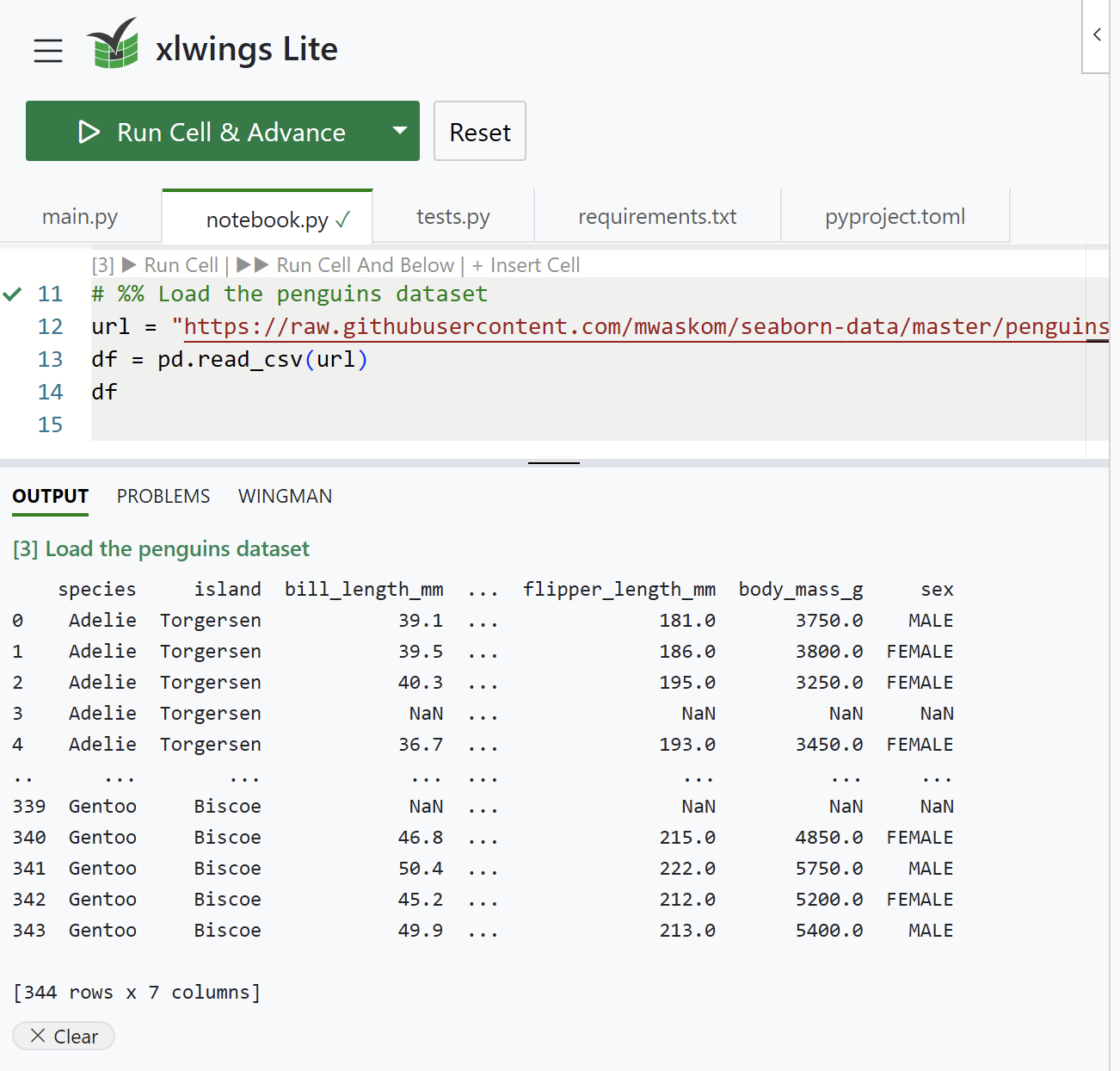
The cell state is shown to the left of the line numbers:

∗	The cell is currently running.
✓	The cell ran successfully.
✕	The cell raised an error.

Unlike Jupyter notebooks, the numbers ([1], [2], etc.) indicate each cell’s current position and don’t increase with every run. This allows you to easily connect the output from the Output pane with the respective cell.

Like Jupyter, the notebook automatically displays the value of the last expression in a cell. In the screenshot above, a cell whose last line is just df shows the DataFrame in the output pane—you don’t need to call print().

All cells share one Python namespace, so variables, imports, and functions defined in one cell are available in other cells, just as they are in Jupyter notebooks.

View in Excel

After running a cell, you can right-click on a variable name and select View in Excel (new sheet). This writes the variable’s data to a new sheet named after the variable, e.g. df. Viewing the same variable again adds another sheet with a counter (df2, df3, etc.). If the variable is a pandas or Polars DataFrame, it will be formatted as an Excel table:

Running cells

You can run cells via the run button, cell actions, or keyboard shortcuts:

Run button

The dropdown lets you choose what the button does:

Run Cell: run the active cell.
Run Cell & Advance: run the active cell, then move the cursor to the next cell.
Reset & Run All: reset the notebook session and run every cell from the top.

There’s also a Replace output toggle that controls whether running a cell replaces the previous output (default) or appends the new output below it. Reset & Run All always clears the previous output because it resets the notebook session.

Cell actions

Each cell shows a set of clickable links above it:

▶ Run Cell: run just this cell.
▲ Run Above: run every cell above this one (not including this cell).
▼ Run Cell And Below: run this cell and every cell below it.
＋ Insert Cell: add a new empty # %% cell right after this one.
－ Delete Cell: remove this cell.

Keyboard shortcuts

The following keyboard shortcuts are available:

Shift + Enter: run the current cell and advance, i.e., move the cursor to the next cell. If you run the last cell, a new empty cell is added at the end and the cursor moves into it (just like Jupyter).
Ctrl + Enter (Windows) / Cmd + Enter (macOS): run the current cell without advancing.
F5: run the action currently selected in the Run button.

Plots

Notebooks support the following plotting libraries:

Here are a few examples for each library:

Matplotlib

import matplotlib.pyplot as plt

plt.plot([1, 2, 3, 4, 5])

or, using the object-oriented interface:

import matplotlib.pyplot as plt

fig, ax = plt.subplots()
ax.plot([1, 2, 3, 4, 5])

Seaborn

Both the figure-level and axes-level functions work:

import seaborn as sns

tips = sns.load_dataset("tips")
sns.relplot(data=tips, x="total_bill", y="tip", hue="time")

or, using the objects interface:

import seaborn as sns
import seaborn.objects as so

tips = sns.load_dataset("tips")
so.Plot(tips, x="total_bill", y="tip").add(so.Dot())

Plotly

import plotly.express as px

df = px.data.iris()
px.scatter(df, x="sepal_width", y="sepal_length", color="species")

import plotly.express as px

df = px.data.iris()
fig = px.scatter(df, x="sepal_width", y="sepal_length", color="species")
fig.show()

Bokeh

from bokeh.plotting import figure

p = figure(title="Simple line example", x_axis_label="x", y_axis_label="y")
p.line([1, 2, 3, 4, 5], [6, 7, 2, 4, 5], legend_label="Temp.", line_width=2)
p

from bokeh.plotting import figure, show

p = figure(title="Simple line example", x_axis_label="x", y_axis_label="y")
p.line([1, 2, 3, 4, 5], [6, 7, 2, 4, 5], legend_label="Temp.", line_width=2)
show(p)

Altair

import altair as alt
from altair.datasets import data

cars = data.cars()
alt.Chart(cars).mark_point().encode(
    x="Horsepower",
    y="Miles_per_Gallon",
    color="Origin",
).interactive()

Plotnine

from plotnine import aes, geom_point, ggplot
from plotnine.data import mtcars

ggplot(mtcars, aes("wt", "mpg", color="factor(gear)")) + geom_point()

xy

import xy

xy.line_chart(xy.line([1, 2, 3, 4, 5], [120, 180, 165, 240, 310]))

Note

Requires Pyodide 314.0.0 or later.

Top-level async/await support

Notebooks allow you to use await directly at the top level of a cell; you don’t need to wrap your code in an async function as required by regular Python files (e.g., main.py):

import httpx  # add httpx to requirements.txt

async with httpx.AsyncClient() as client:
    response = await client.get("https://api.github.com/repos/xlwings/xlwings")
response.json()["stargazers_count"]

Working with the Excel object model

In notebooks, it is recommended to work with the async API:

Sync API: The whole workbook is loaded the moment you call xw.books.active. With large worksheets, this can get slow or even run out of memory, and values can be outdated by the time you call myrange.value:
```
import xlwings as xw

book = xw.books.active
data = book.sheets[0]["A1:B2"].value
```
data represents the state of the Excel values when you called xw.books.active.
Async API (recommended): Cell values are loaded on demand. This is faster for large workbooks as only the specified data is loaded. On top of that, the values always correspond to the current state in Excel:
```
import xlwings as xw

book = await xw.books.get_active()
data = await book.sheets[0]["A1:B2"].get_value()
```
data represents the state of the Excel values when you called get_value().

Before running a cell, the current state (except for cell values) is updated automatically. If you need to get the current state mid-cell, run:

await book.load()

Writes to Excel are flushed automatically at the end of each cell, so you’ll see changes appear in the sheet as soon as the cell finishes running. If you need to flush data mid-cell, you can do it explicitly:

await book.flush()

Migrating from Python in Excel to xlwings Lite

You can migrate formulas from Microsoft’s Python in Excel by going to Source files > Import from Python in Excel. This scans the workbook for =PY() formulas, converts them into notebook cells, and writes them to a notebook called imported.nb.py.

An example notebook

# %% Imports
import pandas as pd
import seaborn as sns
import xlwings as xw

# %% Get the book object (Async API)
book = await xw.books.get_active()

# %% Load the penguins dataset
url = "https://raw.githubusercontent.com/mwaskom/seaborn-data/master/penguins.csv"
df = pd.read_csv(url)
df

# %% Write df to a new sheet
sheet = book.sheets.add()
sheet["A1"].value = df.dropna()
sheet.activate()

# %% Read back from Excel (Async API)
data = await sheet["A1"].options(pd.DataFrame, expand="table").get_value()
data

# %% Plot
sns.jointplot(data=data, x="flipper_length_mm", y="bill_length_mm", hue="species")